Predictive analytics using SAP Design Studio and SAP HANA – Part 1

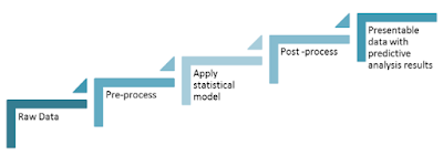
With advanced analytics finding a place in every business function, scripting and programming is too much of a hassle when you are bound by deadlines and tough competition. This is where SAP makes a difference by providing a minimal scripting approach to predictive analytics.
This is a two-part blog where part 1 discusses the fundamentals of SAP HANA PAL & HANA flowgraphs and part 2 discusses how flowgraphs can be integrated with SAP Design Studio to derive actionable insights on the fly.

SAP HANA PAL – Predictive Analytics Library, which is a part of HANA AFL (Application Functions Library) is a large collection of functions to implement predictive modelling. These are the same set of functions that are made available in SAP Predictive Analytics Expert Mode when connecting to a HANA data source. Earlier on, these functions could be used by means of a several-step process using SQL scripts – manually creating all of the artefacts required.

Since HANA SPS 6, things have gotten a lot easier. PAL functions can now be consumed using HANA AFM (Application Function Modeler) – what I would call a drag and drop interface to build complex stored procedures. HANA Flowgraphs are development artefacts which get activated as store procedures, which can then be consumed in other applications, or simply be scheduled to run the job every other day.

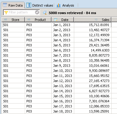
Let’s build a simple flowgraph to understand  how things work. Let’s take the case of a simple sales forecast based on historical trend. I have a table which contains daily sales data of a small retail chain which has 4 stores (S01, S02, S03, S04) in a particular region. For the sake of simplicity, I have chosen 4 top-selling products (P01, P02, P03, P04) of the chain. So we have 4 Stores, 4 Products and the daily sales values of each of these combinations.

Image-1: Sample data in consideration

First, we are going to forecast the overall sales of all stores and products put together. A little analysis of the data tells us that there is a seasonal pattern in the data with a similar pattern repeating every year along with a slight increasing trend and cyclicity. Hence, we will use the Triple Exponential smoothing model from PAL. The flowgraph that we built can be seen below.

Image-2: Flowgraph model

In this case, we aggregate the daily sales over all stores and products to get overall sales numbers for each day of the year, using the aggregation node. Following this, the data needs to be manipulated to a form that is acceptable to the algorithm node. The data is passed through the algorithm to get forecasted values which is then post-processed to a presentable form and written back to a table.

Image-3: Flowgraph development workflow

Image-4: Flowgraph output table

What goes on in the background?

Each node in the flowgraph is transformed into a SQL statement and the entire statement executes as a stored procedure. The predictive algorithm node is executed as a stored procedure call to another procedure which contains the PAL Function call for the data being processed. The properties and configuration of each node and each connection (arrow from one node to the other) can be modified using the Properties View in the AFM. The meta-data information such as the model configuration parameters, input and output table signatures, are stored as catalog objects once the flowgraph is activated.

The activation of a flowgraph triggers the generation of a number of catalog objects.

1. Stored procedure in AFLLANG that calls the PAL Function
2. A wrapper procedure that incorporates all of the data manipulation steps in the flowgraph as nodes with the help of table variables, and also calls the AFLLANG procedure.
3. A number of table types depending on the predictive algorithm used.
4. Parameter tables which were used to define predictive algorithm properties.
5. Write-back tables (if any)

Image-5 & 6: Procedures generated by the flowgraph

While this is a simple example, flowgraphs can be made quite complex and several kinds of analyses can be performed. Some examples include running multiple algorithms on the same data set using a single flowgraph, model comparison, error calculations with the help of the wide range of algorithms and data processing nodes in the AFM. In addition, custom models can be built using R to suit specific use cases.

Extending Flowgraphs to SAP Design Studio

A typical real-life situation would be a lot more complex than the simple example that we just explored. One of them would be to provide this information in a consumable format to the business users so they can put the analytics to use and make informed decisions. Next would be to provide interactivity and allow users to modify various parameters such as dynamically changing the stores and products selected, modifying model parameters to get the most optimal fit and so on. In the next blog, you can read on how to work through some of these complexities taking SAP Design Studio as an example.

Source: scn.sap.com