Simple Linear Regression Python enjoy….

Once again I am writing this because of the motivation i am receiving from one of the most important course running @openSAP Introduction to Statistics and i am sure many of us are the active participant of that ,this resulted in writing this stuff on linear regression.

Regression: In statistical modeling, regression analysis is a set of statistical processes for estimating the relationships between a dependent variable and one or more independent variables. Wikipedia

Introduction: We have two major type of ML Algorithms which are classification and regression.

Classification focus mainly on predicting the class(known labels) – training , testing and prediction is done in this technique.

Here we go for regression and regression analysis :

Uses – Mostly used for forecasting and finding out cause and effect relationship between variables.

Ex– Grades in Study will decrease if student is spending more time on social media So, if X = Spent time on Facebook and Y = Study Grades.

Increase in X will result Decrease in Y hence it is negative relationship between X & Y.

Regression analysis is our topic we are discussing here – focus mainly on predicting a continuous number > consider the below salary observations for experienced SAP professionals

Exp (Yrs)	Salary($)
5	100K
4	80K
3	60K
6	110K
7	120K

from above we can say increase in experience result’s increase in salary it clearly states that one variable is dependent on another variable.

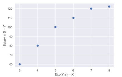
let’s plot this. Our goal is to fit a straight into this & then later use that for predicting the salary based on exp.one can easily see this from the graph that a increase in experience is resulting a increase in salary so if we find out the equation for that then we can easily predict what could be the salary of person having some(Number of Years) exp.let’s do this.

X- Axis – representing the experience in Yrs.

Y- Axis – representing the Salary in $

Important Point – An easy way to distinguish between classification and regression tasks is to ask whether there is some kind of ordering or continuity in the output. if there is an ordering, or a continuity between possible outcomes , then problem is a regression problem.

In this case of Simple Linear regression we will be working with two variables just , one is dependent and other is independent.

Suppose if we do have only one variable and need to find out what’s the next value which can come the simple answer is the mean value of that particular column.

Linear regression mainly tells us how strong the relationship between two variables, before applying this technique check correlation coefficient between these two variables.

execute this in jupyter cell  –

Import numpy as np

x = [3,4,5,6,7 ,8]

y = [60 , 80 , 100 , 110 , 120, 122]

np.corrcoef([x,y])

Coefficient value – 0.96445475 this clearly states the variables are strongly correlated hence go ahead for linear regression application

x – dependent variable (Exp in Yrs)

y – independent variable (Salary in $)

One variable is function of other variable, means value of dependent variable is a function of independent variable.

y = f(x)

salary = f(exp.)

How salary is getting calculated from experience is the function we need to find out for further prediction/forecasting, and linear regression is a Bi-variate statistics where we are dealing with two variables.

First we will look at below formula for calculating the these two variables and then summation and minimization of that

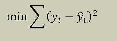
Yi – Observed value of dependent variable (it is actual salary recorded/collected with exp.)

Yi(hat) – estimated predicted values of the dependent variable (predicted salary for exp.)

The goal is to minimize the sum of the squared differences between the observed value for the dependent variable for the dependent (Yi) and the estimated/predicted value of the dependent variable Yi(hat) and it is provided by regression line.

let’s take Exp. = 3 Yr , Actual Salary – 60K, Predicted Salary = 62K

Min (62-60)**2 = MIN(4) = 4 So goal of regression analysis is to fit the best line which can predict the closest value based on the data provided to it and minimize the distance between actual and predicted value , if distance is large then it wouldn’t be called a best fit.

Note: Always try to plot the data which will help you to understand what is happening in case of fitting the line means you can see in the graph how the line can be fitted into these values.

Find mean values for these two variables x & y.

mean_x = np.mean(x)

mean_y = np.mean(y)

mean_x = 5.5

mean_y = 98.66

centroid of line is (mean_x , mean_y) i.e. (5.5 , 98.66) –

Why this centroid is important, the best fit or least squared regression line must go through this point.

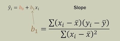
next task is to find out the slope of the regression line – Y(hat) = mx + b

m – slope of the line

b – Intercept from the Y axis means at Y axis where the line will start , b = Y(bar) – mX(bar)

Now calculate these values to find out the slop of the line , let’s go back to jupyter notebook –

◉ Calculate Mean

mean_x = np.mean(x)

mean_y = round(np.mean(y),2)

n = np.size(x)​

◉ X_MINUS_XBAR = []  ##(X-X(bar))

Y_MINUS_YBAR = []  ##(Y-Y(bar))

X_BAR_Y_BAR = []   ##(X-X(bar) * (Y-Y(bar)))

X_MINUS_XBAR_SQUARE = []  ##(X - X(bar)) * (X - X(bar)) 

◉ Calculate (X – X(bar)) & (Y – Y(bar))

for i in range(len(x)):

    X_MINUS_XBAR.append(round(x[i] - mean_x))

    Y_MINUS_YBAR.append((round(y[i] - mean_y) , 2))​

◉ Calculate (X- X(bar)) * (Y – Y(bar))

covar = 0.0

for i in range(len(x)):

    covar += (x[i] - mean_x) * (y[i] - mean_y)

    X_BAR_Y_BAR.append(((x[i] - mean_x) * (y[i] - mean_y)))​

◉ Calculate Square for (X – X(bar))

for i in range(len(X_MINUS_XBAR)):

    X_MINUS_XBAR_SQUARE.append(X_MINUS_XBAR[i] ** 2)​

◉ Summation for (X- X(bar)) * (Y – Y(bar)) & (X – X(bar)) Square

SUM_X_BAR_Y_BAR = sum(X_BAR_Y_BAR)

SUM_X_MINUS_XBAR_SQUARE = sum(X_MINUS_XBAR_SQUARE)​

◉ Slope Calculation

m = SUM_X_BAR_Y_BAR / SUM_X_MINUS_XBAR_SQUARE ​

◉ Calculate Y – Intercept

#Calculate the y-intercept 𝑏 = 𝑦(bar) − 𝑚𝑥(bar)

b = mean_y -  m*mean_x​

◉ We are done now and we got first best fit line  –

x_new = 0.0

y_new = m*x_new + b ​

◉ y_new =  13.75*x_new + 23.045

Now we can use this best fit line for further prediction of the values

This is our data which we have used for finding the best fit line , now we can test this with new values and old as well –

this snippet displays the predicted values for dataset –

for i in x:

    x_new = i

    print(m*x_new+b)

64.295

78.045

91.795

105.545

119.295

133.04500000000002

Also try for new values of experience and it will give the closest salary which a consultant can get

x_new = 10

print(m*x_new+b)

x_new = 11

print(m*x_new+b)

x_new = 20

print(m*x_new+b)

160.54500000000002

174.29500000000002

298.045

reg_line = [ (m*x_val) +b for x_val in x] # Draw regression Line 

plt.scatter(x,y,color="red")          ## Add plotting details

plt.plot(x,reg_line)

plt.ylabel("Independent variable")

plt.xlabel("Dependent variable")

plt.title("Regression Analysis")

plt.show()

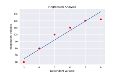
Here is the final outcome of our regression analysis , i think i am done with the basic linear regression analysis , but learning is not yet finished , i will be writing the next article only on root mean square error elaboration.