Just a short recap: Instead of predicting outcomes based on exact coordinates, we will predict the taxi destination base on the area (i.e. hexagonal cell) where the taxi is departing.
When looking at hexagonal cells also for destination areas of the taxi we eventually deal with a multiclass classification problem, where each hexagonal cell (i.e. its ID value) is one target class. HANA’s Automated Predictive Library offers a GradientBoostingClassifier, which is capable of doing multiclass classifications.
Data Preparation and Enhancement
However, there is one limitation of the GradientBoostingClassifier that we have to deal with: It supports a maximum of 100 target classes. We can easily spot, that our reference grid contains more than 1300 potential target areas.
SELECT COUNT(*) FROM REFGRID -- Result: 1347
So, how do we handle this? Taxis are often going to the same areas. In our preceding analysis we already identified the hotspots of Porto in terms of taxi pickups and dropoffs. And we have seen that there are many areas with just a very low number of trips arriving or departing.
What would be the impact of only predicting the top 100 destinations? We can check which percentage of our overall trips are arriving in the top 100 cells with the following nested statement:
SELECT SUM(NTRIPS) AS TOP100_LOC, 100 * SUM(NTRIPS) / (SELECT COUNT(*) FROM TAXI) AS PERCENTAGE
FROM
(
SELECT TOP 100 HEXID, COUNT(*) as NTRIPS
FROM TAXI
LEFT JOIN REFGRID ON ENDPOINT.ST_WITHIN(HEXCELL) = 1
GROUP BY HEXID
ORDER BY COUNT(*) DESC
)
As a result, we see that less than 10% of the trips are arriving in other locations. This means a model predicting the top 100 destinations would be applicable for more than 90% of the trips. For the remainder of 10% we would, of course, always predict an incorrect destination. But since these are rare destinations the predication probably would have been hard anyway.
Ok, so we are going to predict the 100 most frequent destination areas.
To make the prediction more interesting we will furthermore incorporate the first 10 locations of the taxi trajectory. This can give us an idea of which direction the taxi is heading to. For the operator in our real-world scenario this would still be a sufficient heads-up for trips, which are not ultra-short.
Based on the first 10 locations in the trip, we would like to add the following features to our training dataset:
1. COMPASS = Direction the taxi is heading to (N, NE, E, SE, S, SW, W, NW)
We will pretend the first point of the trajectory is in the center of a circle and the tenth point on its edge. Based on that we calculate the compass direction. Please note that the usage of “ACOS(0)” is just a hack to get Pi.
0.5 * atan2(SHAPE.ST_POINTN(10).ST_Y() - STARTPOINT.ST_Y(), SHAPE.ST_POINTN(10).ST_X() - STARTPOINT.ST_X())/acos(0)
2. COMPASS_DIST = The bee-line distance that the taxi drove within the first 10 points of the trajectory.
The idea is to detect if the taxi quickly entered a main road or drove along some small alleys.
STARTPOINT.ST_DISTANCE(SHAPE.ST_POINTN(10))
To add those features to our dataset, we can issue the following statement, which also categorizes the compass direction based on the above calculated value.
ALTER TABLE TAXI ADD (COMPASS NVARCHAR(2));
ALTER TABLE TAXI ADD (COMPASS_DIST INTEGER);
UPDATE TAXI T SET
COMPASS =
CASE
WHEN 1 - ABS(D.DIR) <= 0.125 THEN 'W'
WHEN ABS(0 - D.DIR) <= 0.125 THEN 'E'
WHEN ABS(0.5 - D.DIR) <= 0.125 THEN 'N'
WHEN ABS(-0.5 - D.DIR) <= 0.125 THEN 'S'
WHEN ABS(0.25 - D.DIR) < 0.125 THEN 'NE'
WHEN ABS(0.75 - D.DIR) < 0.125 THEN 'NW'
WHEN ABS(-0.25 - D.DIR) < 0.125 THEN 'SE'
WHEN ABS(-0.75 - D.DIR) < 0.125 THEN 'SW'
ELSE NULL
END,
COMPASS_DIST = STARTPOINT.ST_DISTANCE(SHAPE.ST_POINTN(10))
FROM
TAXI T,
(
SELECT TRIP_ID, 0.5 * atan2(SHAPE.ST_POINTN(10).ST_Y() - STARTPOINT.ST_Y(), SHAPE.ST_POINTN(10).ST_X() - STARTPOINT.ST_X())/acos(0) AS DIR
FROM TAXI
WHERE SHAPE.ST_NUMPOINTS() > 10
) D
WHERE T.TRIP_ID = D.TRIP_ID;
Training the Gradient Boosting Model
Well, let’s construct a dataset with 75000 sample trajectories divided into training dataset (80%) and test dataset (20%). To do this we will use the HANA built-in window function RANDOM_PARTITION. The second part of the nested SQL statement we have already seen earlier when selecting the top 100 destinations.
SELECT *, RANDOM_PARTITION(0.8, 0.0, 0.2, 0) OVER (ORDER BY STARTTIME) AS SET_NUM
FROM
(
SELECT TOP 75000
TRIP_ID,
CALL_TYPE,
DAY_TYPE,
STARTTIME,
COMPASS,
COMPASS_DIST,
a.HEXID AS START_HEXID,
b.HEXID AS END_HEXID
FROM TAXI
LEFT JOIN REFGRID a ON STARTPOINT.ST_WITHIN(a.HEXCELL) = 1
LEFT JOIN REFGRID b ON ENDPOINT.ST_WITHIN(b.HEXCELL) = 1
WHERE
COMPASS IS NOT NULL
AND b.HEXID IN
(
SELECT TOP 100 HEXID
FROM TAXI
LEFT JOIN REFGRID ON ENDPOINT.ST_WITHIN(HEXCELL) = 1
GROUP BY HEXID
ORDER BY COUNT(*) DESC
)
ORDER BY RAND()
)
The double use of randomization may seem confusing first. We use “order by rand()” in combination with “top 75000” to randomly pick 75000 samples. These samples we then randomly divide into training and test datasets by using “random_partition()”.
The resulting dataset looks like the following, where END_HEXID is the target variable of our model and SET_NUM determines if the record belongs to the training dataset (SET_NUM = 1) or the test dataset (SET_NUM = 3).
Finally, we are ready to train our gradient boosting model. On my laptop with HANA Express the training lasts around 6 minutes. So take your time and grab a coffee….. or espresso, better grab an espresso.
When using the hana_ml client for Python, the model training will be triggered from within Python. However all calculations are pushed down to the database in the background and data does not get transferred to the client.
gb_model.fit(
hdf_rides.filter('SET_NUM=1'),
label='END_HEXID',
key = 'TRIP_ID',
features = ['CALL_TYPE', 'DAY_TYPE', 'STARTTIME', 'COMPASS', 'COMPASS_DIST', 'START_HEXID']
)
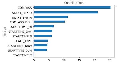
After having our espresso with a load of sugar we observe the contributing features for our classification model.
plot_feature_importance(gb_model.get_feature_importances()['ExactSHAP'])
The three most important influencing factors for determining the destination of a taxi are:
1. The direction the taxi is heading to.
2. The pickup area.
3. The hour of day.
This makes sense – especially the influence of the daytime is expected as trips at around 8pm are probably more likely to end in a bar or restaurant and trips after midnight are more likely to end in suburbs, where people are living.
Evaluate Model Performance
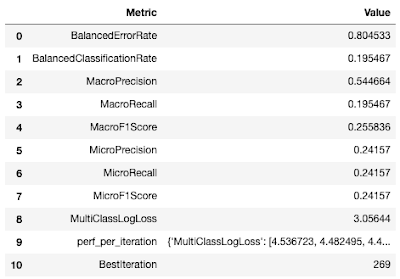
Of course, we can retrieve statistical measures for our model from APL by issuing:
gb_model.get_performance_metrics()
However, this time we want to evaluate the model slightly different. Since we clustered our locations by hexagons we may have some “near-misses” at the edge of the hexagons. The above performance measurements only reflect if we predicted the exact correct target hexagon and it does not include geospatial proximity measures.
To have some data to work with, we will do predictions based on our test dataset of 15000 records.
hdf_predict = gb_model.predict(hdf_rides.filter('SET_NUM=3'))
For each predicted record we now have the correct target hexagon as well as the id of the predicted target hexagon. To evaluate geospatial proximity we need to join the geometry data from our reference grid back to the result table.
hdf_predict_refgrid = hdf_predict.join(
conn.table('REFGRID'),
'TRUE_LABEL = HEXID',
select=[('TRIP_ID'), ('TRUE_LABEL'), ('PREDICTED'), ('PROBABILITY'), ('HEXCENTROID', 'TRUE_CENTROID')]
)
hdf_predict_refgrid = hdf_predict_refgrid.join(
conn.table('REFGRID'),
'PREDICTED = HEXID',
select=[('TRIP_ID'), ('TRUE_LABEL'), ('PREDICTED'), ('PROBABILITY'), ('TRUE_CENTROID'), ('HEXCENTROID', 'PREDICTED_CENTROID')]
)
The resulting dataframe looks like the following, where TRUE_CENTROID and PREDICTED_CENTROID are the centroid points of the respective hexagonal cells/areas. We can see, that APL even added a probability field to the output with which we can determine how likely the predicted location is according to the model.
Based on that, we can calculate the average distance between the predicted and the true centroids.
hdf_predict_refgrid = hdf_predict_refgrid.select('*', ('TRUE_CENTROID.ST_DISTANCE(PREDICTED_CENTROID)', 'DIST'))
hdf_predict_refgrid.agg([('AVG', 'DIST', 'AVG_DIST')]).collect()
So on average we are predicting within a range of 2.6 km. To set this into relation we need to know the diameter of our hexagonal cells.
SELECT TOP 1
HEXCELL.ST_EXTERIORRING().ST_POINTN(1).ST_DISTANCE(HEXCELL.ST_EXTERIORRING().ST_POINTN(4)) AS HEX_DIAMETER
FROM REFGRID
This means due to our spatial binning we can anyhow only do predictions within a range of 1 km. So how many of our predictions are either in the correct target cell or in one of its neighbouring cells? Based on the diameter, we can query the centroids which are in a 1.1km range.
tp_prediction = hdf_predict_refgrid.filter('DIST < 1100').count()
print('%s%%' % (100 * tp_prediction / hdf_predict_refgrid.count()))
We can see, that based on this measurement we predict one third (33.9% in my case) of the trips correctly.
That sounds good, but we should compare this result to a proper baseline. What would happen, if we simply always predict the hexagonal cell with most overall taxi activity? If we only have one guess, this one would probably be good.
We can determine the most frequently visited cell and do the ‘prediction’ as follows.
hdf_top_destination = conn.sql('''
SELECT TOP 1 HEXID, HEXCENTROID
FROM TAXI
LEFT JOIN REFGRID ON ENDPOINT.ST_WITHIN(HEXCELL) = 1
GROUP BY HEXID, HEXCENTROID
ORDER BY COUNT(*) DESC
''')
hdf_predict_frequent = hdf_predict_refgrid.join(
hdf_top_destination,
"1=1",
select=[('TRIP_ID'), ('TRUE_LABEL'), ('PREDICTED'), ('PROBABILITY'), ('TRUE_CENTROID'), ('PREDICTED_CENTROID'), ('HEXCENTROID', 'FREQUENT_CENTROID')]
).select(
'*', ('TRUE_CENTROID.ST_DISTANCE(FREQUENT_CENTROID)', 'FREQUENT_DIST')
)
So, how does our model compare against this ‘majority vote’ as a baseline?
tp_majority = hdf_predict_frequent.filter('FREQUENT_DIST < 1100').count()
print('%s%%' % (100 * (tp_prediction - tp_majority) / hdf_predict_refgrid.count()))
With our model we are still 10% better than with with the baseline. Our model predicted (in my case) 5085 out of 15000 trips correctly, whereas the baseline majority vote predicted only 3568 out of 15000 trips correctly.
Finally, we can configure the APL to also output the probabilities of all other hexagonal clusters, which have not been predicted as a destination.
gb_model.set_params(extra_applyout_settings={'APL/ApplyExtraMode': 'AllProbabilities'})
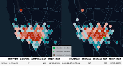
This data we can use to visualize one scenario:
◉ On the left side we can see the probability distribution as well as the predicted destination cell in case we are starting a taxi ride westwards from Campanha train station at 8am in the morning.
◉ In the right picture, we see the same trip just starting at 8pm in the evening and going northeastwards.
Looking at the probability distribution we can tell that the center of the city is a likely destination in any case (independent of time and direction). However for the westwards-variant we do not see any high probabilities in the eastern part of the city and the probability that the trip goes to the airport is significantly higher. For the trip heading northeast we see a higher probability for destinations in the northeast as well as a lower probability for the airport and destinations at the seaside.
As a by-catch we can also nicely see in the visualization, that our top 100 destination areas essentially cover the urban core of Porto.


No comments:
Post a Comment