When we collect data at a measurable interval such as time, the data is called series data. Analysis of series data allows you to draw meaningful conclusions and predictions from the patterns and trends present in the values. Examples of time series are sensor data generated by IoT, weather station, daily closing value of the stock ticker etc.
Series table operations are performed like column table operations with a few features to consider.
SERIES clause of the CREATE COLUMN TABLE statements which support both equidistant and non-equidistant data
Syntax:
CREATE [ <table_type> ] { <table_name> }
SERIES ([<series_key>]
[<series_equidistant_definition>]
[<series_minvalue>]
[<series_maxvalue>]
<series_period> [<alternate_series>] )
EQUIDISTANT INCREMENT BY INTERVAL
MISSING ELEMENTS NOT ALLOWED
Machine readings and temperature are two examples for equidistant series as following. data is read and captured with certain interval during fixed period
CREATE COLUMN TABLE TIMESERIES.MACHINE_READINGS (
SENSOR VARCHAR(15),
TIMER TIMESTAMP,
READING DECIMAL(10,2)
)
SERIES (
SERIES KEY(SENSOR)
PERIOD FOR SERIES(TIMER)
EQUIDISTANT INCREMENT BY INTERVAL 1 MINUTE
MISSING ELEMENTS NOT ALLOWED
MINVALUE '2015-01-01 00:01:00'
MAXVALUE '2015-12-31 23:59:00'
);
CREATE COLUMN TABLE TIMESERIES.MACHINE_TEMPERATURE (
SENSOR VARCHAR(15),
TIMER TIMESTAMP,
TEMPERATURE DECIMAL(10,2)
)
SERIES (
SERIES KEY(SENSOR)
PERIOD FOR SERIES(TIMER)
EQUIDISTANT INCREMENT BY INTERVAL 1 HOUR
MISSING ELEMENTS NOT ALLOWED
MINVALUE '2015-01-01 00:00:00'
MAXVALUE '2015-12-31 23:00:00'
);
DELETE FROM TIMESERIES.MACHINE_READINGS;
INSERT INTO TIMESERIES.MACHINE_READINGS (
SELECT
'MACHINE_1',
GENERATED_PERIOD_START,
ROUND(20+RAND()*20,1)
FROM
SERIES_GENERATE_TIMESTAMP('INTERVAL 1 MINUTE', '2015-01-01 00:01:00', '2015-01-31 23:59:00')
);
DELETE FROM TIMESERIES.MACHINE_TEMPERATURE;
INSERT INTO TIMESERIES.MACHINE_TEMPERATURE (
SELECT
'MACHINE_1',
GENERATED_PERIOD_START,
30 + ROUND(RAND()*6,1)
FROM
SERIES_GENERATE_TIMESTAMP('INTERVAL 1 HOUR', '2015-01-01 00:00:00', '2015-01-31 23:00:00')
);
EQUIDISTANT INCREMENT BY INTERVAL
MISSING ELEMENTS ALLOWED
Machine readings are captured from sensor, in reality sensors may have downtime or disorder this could cause data element missing
CREATE COLUMN TABLE TIMESERIES.MACHINE_READINGS
(
SENSOR VARCHAR(15),
TIMER TIMESTAMP,
READING DECIMAL(10,2)
)
SERIES
(
SERIES KEY(SENSOR)
PERIOD FOR SERIES(TIMER)
EQUIDISTANT INCREMENT BY INTERVAL 1 HOUR
MISSING ELEMENTS ALLOWED
MINVALUE '2015-01-01 00:00:00'
MAXVALUE '2015-12-31 23:00:00'
);
EQUIDISTANT PIECEWISE
A degree of regularity without being equidistant across the entire dataset can be represented using equidistant piecewise tables
The equidistant piecewise specification can only be used in CDS; it cannot be used to create a table with the SQL command CREATE TABLE.
1. The period includes one column; there is no support for interval periods.
2. There is no support for missing elements.
3. The type of the period column must map to the one of the following types: DATE, SECONDDATE, or TIMESTAMP.
context MySeriesContext
{
entity MySeriesEntity
{
key setId : Integer;
t : UTCTimestamp;
value : Decimal(10,4);
series
(
series key (setId)
period for series (t)
equidistant piecewise
)
};
NOT EQUIDISTANT
Often, source data will be non-equidistant. In order to do further analysis, it need to be converted to an equidistant grid first.
For stock ticker history you can store it as NOT EQUIDISTANT considering stock market close on weekend and holiday. Alternatively you can store the ticker data as EQUIDISTANT MISSING ELEMENT ALLOWED so closed days will be treated as missing element.
You can download the sample stock ticker history data from quandl.com
CREATE COLUMN TABLE "TIMESERIES"."US_STOCK_PRICES"
(
"TICKER" NVARCHAR(15),
"TICK_DATE" DATE,
"OPEN" DECIMAL(15,6),
"HIGH" DECIMAL(15,6),
"LOW" DECIMAL(15,6),
"CLOSE" DECIMAL(15,6),
"VOLUME" DECIMAL(12,1),
"DIVIDEND" DECIMAL(6,2),
"SPLIT" DECIMAL(4,1),
"ADJ_OPEN" DECIMAL(33,15),
"ADJ_HIGH" DECIMAL(33,15),
"ADJ_LOW" DECIMAL(33,15),
"ADJ_CLOSE" DECIMAL(33,15),
"ADJ_VOLUME" DECIMAL(12,1)
)
SERIES
(
SERIES KEY ("TICKER")
PERIOD FOR SERIES("TICK_DATE")
NOT EQUIDISTANT
);
For series data you can store in normal columnar table but SAP have optimal data structure and memory saving with SERIES clause . For series with EQUIDISTANT memory savings could reach 88% compared to normal columnar table.
When data is first inserted into an equidistant piecewise series table, use this clause to reorder rows to maximize compression.
Alter column table SERIES REORGANIZE
SERIES_TABLES view
The SERIES_TABLES view contains configuration settings for each series table, such as period and calendar settings, and whether the series table is equidistant.
M_SERIES_TABLES view
The M_SERIES_TABLES view contains statistics on the physical contents of each series table.
SERIES_KEY_COLUMNS view
The SERIES_KEY_COLUMNS view contains the series key column for each series table.
You can generate a complete series according to a definition using the SERIES_GENERATE function
The examples below illustrates different ways to generate series data
SERIES_GENERATE_TIMESTAMP
SELECT * FROM SERIES_GENERATE_TIMESTAMP( ‘INTERVAL 1 HOUR’, ‘2015-01-01 00:00:00′,’2015-01-31 23:00:00’)
SERIES_GENERATE_DATE
SELECT * FROM SERIES_GENERATE_DATE( ‘INTERVAL 1 DAY’, ‘2015-01-01′,’2020-01-01’)
SELECT * FROM SERIES_GENERATE_DATE( ‘INTERVAL 1 MONTH’, ‘2015-01-01′,’2020-01-01’)
Aggregate functions can be used with series data to perform vertical aggregation, and horizontal aggregation.
1. Horizontal aggregation refers to aggregation over longer periods
-- horizontal aggregation, using series_round & round_down, minute to hour
SELECT
SENSOR,
SERIES_ROUND(TIMER, 'INTERVAL 1 HOUR', ROUND_DOWN) AS TIMER_HOUR,
AVG(READING) AS READING_AVG_HOUR
FROM TIMESERIES.MACHINE_READINGS
GROUP BY SENSOR, SERIES_ROUND(TIMER, 'INTERVAL 1 HOUR', ROUND_DOWN);
-- horizontal aggregation, using series_round & round_down, day to month
SELECT min("TICK_DATE") as"TICK_DATE",
first_value("OPEN" order by "TICK_DATE") as"OPEN",
last_value("CLOSE" order by "TICK_DATE") as"CLOSE",
max("HIGH") as "HIGH",
min("LOW") as "LOW",
sum("VOLUME") as"VOLUME"
FROM "TIMESERIES"."US_STOCK_PRICES"
GROUP BY SERIES_ROUND("TICK_DATE", 'INTERVAL 1 MONTH', ROUND_DOWN)
2.Vertical aggregation refers to aggregation across different series.
-- vertical aggregation between readings & temperature tables
SELECT
MT.SENSOR,
MT.TIMER,
(
-- horizontal aggregation, using series_round & round_down, minute to hour
SELECT AVG(MR.READING)
FROM TIMESERIES.MACHINE_READINGS MR
WHERE MR.SENSOR = MT.SENSOR AND
SERIES_ROUND(MR.TIMER, 'INTERVAL 1 HOUR', ROUND_DOWN) = MT.TIMER
) AS READING_AVG_HOUR,
MT.TEMPERATURE
FROM
TIMESERIES.MACHINE_TEMPERATURE MT;
Series table operations are performed like column table operations with a few features to consider.
SQL statements
SERIES clause of the CREATE COLUMN TABLE statements which support both equidistant and non-equidistant data
Syntax:
CREATE [ <table_type> ] { <table_name> }
SERIES ([<series_key>]
[<series_equidistant_definition>]
[<series_minvalue>]
[<series_maxvalue>]
<series_period> [<alternate_series>] )
Scenario 1:
EQUIDISTANT INCREMENT BY INTERVAL
MISSING ELEMENTS NOT ALLOWED
Machine readings and temperature are two examples for equidistant series as following. data is read and captured with certain interval during fixed period
CREATE COLUMN TABLE TIMESERIES.MACHINE_READINGS (
SENSOR VARCHAR(15),
TIMER TIMESTAMP,
READING DECIMAL(10,2)
)
SERIES (
SERIES KEY(SENSOR)
PERIOD FOR SERIES(TIMER)
EQUIDISTANT INCREMENT BY INTERVAL 1 MINUTE
MISSING ELEMENTS NOT ALLOWED
MINVALUE '2015-01-01 00:01:00'
MAXVALUE '2015-12-31 23:59:00'
);
CREATE COLUMN TABLE TIMESERIES.MACHINE_TEMPERATURE (
SENSOR VARCHAR(15),
TIMER TIMESTAMP,
TEMPERATURE DECIMAL(10,2)
)
SERIES (
SERIES KEY(SENSOR)
PERIOD FOR SERIES(TIMER)
EQUIDISTANT INCREMENT BY INTERVAL 1 HOUR
MISSING ELEMENTS NOT ALLOWED
MINVALUE '2015-01-01 00:00:00'
MAXVALUE '2015-12-31 23:00:00'
);
DELETE FROM TIMESERIES.MACHINE_READINGS;
INSERT INTO TIMESERIES.MACHINE_READINGS (
SELECT
'MACHINE_1',
GENERATED_PERIOD_START,
ROUND(20+RAND()*20,1)
FROM
SERIES_GENERATE_TIMESTAMP('INTERVAL 1 MINUTE', '2015-01-01 00:01:00', '2015-01-31 23:59:00')
);
DELETE FROM TIMESERIES.MACHINE_TEMPERATURE;
INSERT INTO TIMESERIES.MACHINE_TEMPERATURE (
SELECT
'MACHINE_1',
GENERATED_PERIOD_START,
30 + ROUND(RAND()*6,1)
FROM
SERIES_GENERATE_TIMESTAMP('INTERVAL 1 HOUR', '2015-01-01 00:00:00', '2015-01-31 23:00:00')
);
Scenario 2:
EQUIDISTANT INCREMENT BY INTERVAL
MISSING ELEMENTS ALLOWED
Machine readings are captured from sensor, in reality sensors may have downtime or disorder this could cause data element missing
CREATE COLUMN TABLE TIMESERIES.MACHINE_READINGS
(
SENSOR VARCHAR(15),
TIMER TIMESTAMP,
READING DECIMAL(10,2)
)
SERIES
(
SERIES KEY(SENSOR)
PERIOD FOR SERIES(TIMER)
EQUIDISTANT INCREMENT BY INTERVAL 1 HOUR
MISSING ELEMENTS ALLOWED
MINVALUE '2015-01-01 00:00:00'
MAXVALUE '2015-12-31 23:00:00'
);
Scenario 3:
EQUIDISTANT PIECEWISE
A degree of regularity without being equidistant across the entire dataset can be represented using equidistant piecewise tables
The equidistant piecewise specification can only be used in CDS; it cannot be used to create a table with the SQL command CREATE TABLE.
1. The period includes one column; there is no support for interval periods.
2. There is no support for missing elements.
3. The type of the period column must map to the one of the following types: DATE, SECONDDATE, or TIMESTAMP.
context MySeriesContext
{
entity MySeriesEntity
{
key setId : Integer;
t : UTCTimestamp;
value : Decimal(10,4);
series
(
series key (setId)
period for series (t)
equidistant piecewise
)
};
Scenario 4:
NOT EQUIDISTANT
Often, source data will be non-equidistant. In order to do further analysis, it need to be converted to an equidistant grid first.
For stock ticker history you can store it as NOT EQUIDISTANT considering stock market close on weekend and holiday. Alternatively you can store the ticker data as EQUIDISTANT MISSING ELEMENT ALLOWED so closed days will be treated as missing element.
You can download the sample stock ticker history data from quandl.com
CREATE COLUMN TABLE "TIMESERIES"."US_STOCK_PRICES"
(
"TICKER" NVARCHAR(15),
"TICK_DATE" DATE,
"OPEN" DECIMAL(15,6),
"HIGH" DECIMAL(15,6),
"LOW" DECIMAL(15,6),
"CLOSE" DECIMAL(15,6),
"VOLUME" DECIMAL(12,1),
"DIVIDEND" DECIMAL(6,2),
"SPLIT" DECIMAL(4,1),
"ADJ_OPEN" DECIMAL(33,15),
"ADJ_HIGH" DECIMAL(33,15),
"ADJ_LOW" DECIMAL(33,15),
"ADJ_CLOSE" DECIMAL(33,15),
"ADJ_VOLUME" DECIMAL(12,1)
)
SERIES
(
SERIES KEY ("TICKER")
PERIOD FOR SERIES("TICK_DATE")
NOT EQUIDISTANT
);
Memory Optimization
For series data you can store in normal columnar table but SAP have optimal data structure and memory saving with SERIES clause . For series with EQUIDISTANT memory savings could reach 88% compared to normal columnar table.
When data is first inserted into an equidistant piecewise series table, use this clause to reorder rows to maximize compression.
Alter column table SERIES REORGANIZE
System View
SERIES_TABLES view
The SERIES_TABLES view contains configuration settings for each series table, such as period and calendar settings, and whether the series table is equidistant.
M_SERIES_TABLES view
The M_SERIES_TABLES view contains statistics on the physical contents of each series table.
SERIES_KEY_COLUMNS view
The SERIES_KEY_COLUMNS view contains the series key column for each series table.
Series Generation
You can generate a complete series according to a definition using the SERIES_GENERATE function
The examples below illustrates different ways to generate series data
SERIES_GENERATE_TIMESTAMP
SELECT * FROM SERIES_GENERATE_TIMESTAMP( ‘INTERVAL 1 HOUR’, ‘2015-01-01 00:00:00′,’2015-01-31 23:00:00’)
SERIES_GENERATE_DATE
SELECT * FROM SERIES_GENERATE_DATE( ‘INTERVAL 1 DAY’, ‘2015-01-01′,’2020-01-01’)
SELECT * FROM SERIES_GENERATE_DATE( ‘INTERVAL 1 MONTH’, ‘2015-01-01′,’2020-01-01’)
Aggregation
Aggregate functions can be used with series data to perform vertical aggregation, and horizontal aggregation.
1. Horizontal aggregation refers to aggregation over longer periods
-- horizontal aggregation, using series_round & round_down, minute to hour
SELECT
SENSOR,
SERIES_ROUND(TIMER, 'INTERVAL 1 HOUR', ROUND_DOWN) AS TIMER_HOUR,
AVG(READING) AS READING_AVG_HOUR
FROM TIMESERIES.MACHINE_READINGS
GROUP BY SENSOR, SERIES_ROUND(TIMER, 'INTERVAL 1 HOUR', ROUND_DOWN);
-- horizontal aggregation, using series_round & round_down, day to month
SELECT min("TICK_DATE") as"TICK_DATE",
first_value("OPEN" order by "TICK_DATE") as"OPEN",
last_value("CLOSE" order by "TICK_DATE") as"CLOSE",
max("HIGH") as "HIGH",
min("LOW") as "LOW",
sum("VOLUME") as"VOLUME"
FROM "TIMESERIES"."US_STOCK_PRICES"
GROUP BY SERIES_ROUND("TICK_DATE", 'INTERVAL 1 MONTH', ROUND_DOWN)
2.Vertical aggregation refers to aggregation across different series.
-- vertical aggregation between readings & temperature tables
SELECT
MT.SENSOR,
MT.TIMER,
(
-- horizontal aggregation, using series_round & round_down, minute to hour
SELECT AVG(MR.READING)
FROM TIMESERIES.MACHINE_READINGS MR
WHERE MR.SENSOR = MT.SENSOR AND
SERIES_ROUND(MR.TIMER, 'INTERVAL 1 HOUR', ROUND_DOWN) = MT.TIMER
) AS READING_AVG_HOUR,
MT.TEMPERATURE
FROM
TIMESERIES.MACHINE_TEMPERATURE MT;
SQL Analytic Functions
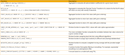
First, Last, Nth Value Aggregate Functions
Changing the time granularity from days to months
SELECT min("TICK_DATE") as"date",
first_value("OPEN" order by"date") as"open",
last_value("CLOSE" order by"date") as"close",
max("HIGH") as"high",
min("LOW") as"low",
sum("VOLUME") as"volume"
FROM "TIMESERIES"."US_STOCK_PRICES"
GROUP BY SERIES_ROUND("TICK_DATE", 'INTERVAL 1 MONTH', ROUND_DOWN)
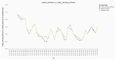
Linear Interpolation & Cubic Spline Interpolation
Replacement of null values by interpolating the gaps and extrapolating any leading or trailing null values. Interpolation can be done by
Linear Interpolation
Use the LINEAR_APPROX function to replace null values in equidistant series data by interpolating the gaps and extrapolating any leading or trailing null values
Syntax:
<linear_approx_function> ::= LINEAR_APPROX (<expression> [, <ModeArgument> [, <Value1Argument> [,
<Value2Argument>]]]) OVER ({ SERIES TABLE <table_schema> [<window_partition_by_clause>]
[<window_order_by_clause>] | SERIES(…) [<window_partition_by_clause>]
[<window_order_by_clause>] | [<window_partition_by_clause>] <window_order_by_clause>})
<expression> ::= <identifier>
CREATE COLUMN TABLE "InterpolationTable" (TS_ID VARCHAR(20), date DAYDATE, val DOUBLE);
INSERT INTO "InterpolationTable" VALUES ('A','2013-09-30', 1);
INSERT INTO "InterpolationTable" VALUES ('A','2013-10-01', 2);
INSERT INTO "InterpolationTable" VALUES ('A','2013-10-02', null);
INSERT INTO "InterpolationTable" VALUES ('A','2013-10-03', 10);
SELECT date, val, LINEAR_APPROX (val, 'EXTRAPOLATION_LINEAR') OVER (PARTITION BY TS_ID ORDER BY date) FROM "InterpolationTable";
Cubic Spline Interpolation
Replaces null values by interpolating the gaps based on calculated cubic splines and linearly extrapolating any leading or trailing null values.
Syntax:
CUBIC_SPLINE_APPROX ( <expression> [, <BoundaryConditionArgument> [, <ExtrapolationModeArgument> [, <Value1Argument> [, <Value2Argument> ] ] ] ] )
[ OVER ( {
SERIES TABLE <series_table> [ PARTITION BY <col1> [,…] [ <window_order_by_clause> ]
| SERIES(…) [ PARTITION BY <col1> [,…] [ <window_order_by_clause> ]
| [ PARTITION BY <col1>[,…] <window_order_by_clause>
} ) ]
CREATE COLUMN TABLE "InterpolationTable"
(ts_id VARCHAR(20), date DAYDATE, val DOUBLE)
SERIES(SERIES KEY(ts_id) PERIOD FOR SERIES(date)
EQUIDISTANT INCREMENT BY INTERVAL 1 DAY MISSING ELEMENTS ALLOWED);
INSERT INTO "InterpolationTable" VALUES ('A','2013-09-29', null);
INSERT INTO "InterpolationTable" VALUES ('A','2013-09-30', 1);
INSERT INTO "InterpolationTable" VALUES ('A','2013-10-01', 2);
INSERT INTO "InterpolationTable" VALUES ('A','2013-10-02', null);
INSERT INTO "InterpolationTable" VALUES ('A','2013-10-03', 10);
INSERT INTO "InterpolationTable" VALUES ('A','2013-10-04', 5);
INSERT INTO "InterpolationTable" VALUES ('A','2013-10-05', null);
SELECT CUBIC_SPLINE_APPROX(val, 'SPLINE_TYPE_NOT_A_KNOT') OVER(SERIES TABLE "InterpolationTable") FROM "InterpolationTable";
Auto Correlation & Cross Correlation
They are used to find periodic pattern in the data, like seasonality.
◉ Auto-correlation looks for periodicity between values of the same series as a function of the time lag between them.
Syntax
AUTO_CORR( <expression>, <maxTimeLag> { <series_order_by_clause> | <order_by_clause> })Auto Correlation example
CREATE COLUMN TABLE correlationTable (TS_ID VARCHAR(10), DATE DAYDATE, VALUE DOUBLE);
INSERT INTO correlationTable VALUES ('A', '2014-10-01', 1);
INSERT INTO correlationTable VALUES ('A', '2014-10-02', 2);
INSERT INTO correlationTable VALUES ('A', '2014-10-03', 3);
INSERT INTO correlationTable VALUES ('A', '2014-10-04', 4);
INSERT INTO correlationTable VALUES ('A', '2014-10-05', 5);
INSERT INTO correlationTable VALUES ('A', '2014-10-06', 1);
INSERT INTO correlationTable VALUES ('A', '2014-10-07', 2);
INSERT INTO correlationTable VALUES ('A', '2014-10-08', 3);
INSERT INTO correlationTable VALUES ('A', '2014-10-09', 4);
INSERT INTO correlationTable VALUES ('A', '2014-10-10', 5);
SELECT TS_ID, AUTO_CORR(VALUE, 8 SERIES (PERIOD FOR SERIES(DATE)
EQUIDISTANT INCREMENT BY INTERVAL 1 DAY MISSING ELEMENTS NOT ALLOWED))
FROM correlationTable GROUP BY TS_ID ORDER BY TS_ID;
◉ Cross-correlation looks for periodicity between values of different series as a function of the time lag between them
CROSS_CORR(<expression1>, <expression2>, <maxLag>
{ <series_orderby> | <order_by_clause> } ).{ POSITIVE_LAGS | NEGATIVE_LAGS | ZERO_LAG }Cross Correlation example
CREATE COLUMN TABLE TSeries( key INTEGER, ts TIMESTAMP, val1 DOUBLE, val2 DOUBLE, PRIMARY KEY(key, ts) )
SERIES( SERIES KEY (key) EQUIDISTANT INCREMENT BY INTERVAL 1 DAY PERIOD FOR SERIES(ts) );
INSERT INTO TSeries VALUES (1, '2014-1-1', 1, 3);
INSERT INTO TSeries VALUES (2, '2014-1-3', 2, 4);
INSERT INTO TSeries VALUES (3, '2014-1-4', 4, 2);
INSERT INTO TSeries VALUES (4, '2014-1-5', 3, 1);
SELECT CROSS_CORR(val1, val2, 10 ORDER BY ts) FROM TSeries;
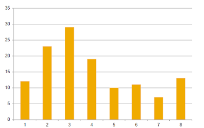
Binning
Binning assigns data values to bins.
Syntax
<binning_function> ::= BINNING( <binning_param> => <expression> [ {, <binning_parameter> => <expression> } … ] )
<binning_param> ::= VALUE | BIN_COUNT | BIN_WIDTH | TILE_COUNT | STDDEV_COUNT
SELECT bin_number, count(bin_number) as cnt
FROM(
SELECT binning(value=> “OPEN”, bin_count=> 8) OVER (ORDER BY “TICK_DATE”) AS bin_number
FROM “TIMESERIES”.”US_STOCK_PRICES_NOT_EQUIDISTANT”
)
GROUP BY bin_number
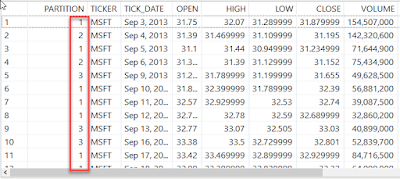
Random Partition
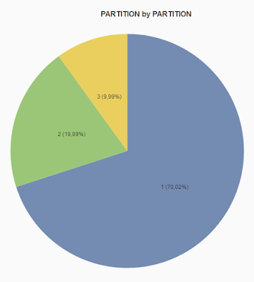
Partitioning divides the input data into three sets, a training, a validation, and a test set that are used in machine learning.
Syntax
RANDOM_PARTITION(<training_set_size>, <validation_set_size>, <test_set_size>, <seed>) <window_specification>
SELECT *, random_partition(0.7, 0.2, 0.1) OVER (PARTITION BY “TICKER” ORDER BY “TICK_DATE”) AS “PARTITION”
FROM “TIMESERIES”.”US_STOCK_PRICES_NOT_EQUIDISTANT”
Discrete Fourier Transform
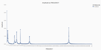
It is used in spectral analysis of series data, e.g. in vibration analysis
Computation uses the FFT algorithm and returns
Syntax
DFT (<column>, <N>
{SERIES( … ) | ORDER BY <col1>, … }).{REAL|IMAGINARY|AMPLITUDE|PHASE}
1.Amplitude / phase
2.Real part / imaginary part
Example:
SELECT ordinality AS "frequency", "amplitude"/4096 AS "amplitude"
FROM unnest((
SELECT dft("amplitude", 4096 order by "ts").amplitude
FROM"vibration"
)) WITH ORDINALITY AS tt(amplitude)
Filtering Series Data
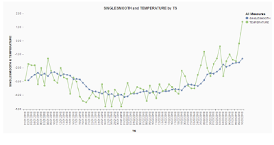
Use the SERIES_FILTER window function to returns value from an equidistant series, with the specified filter applied. The following example returns values filtered by the SINGLESMOOTH and DOUBLESMOOTH filters.
Syntax
SERIES_FILTER(<filter_parameter> => <expression> [{, <filter_parameter> => <expression>} … ])
OVER (
[<series_definition> | <series_reference>]
[<window_partition_by_clause>]
[ORDER BY <window_order_by_expression>]
[ <window_frame_clause> ]
)
<filter_parameter> ::= VALUE | METHOD_NAME | ALPHA | BETA
Example:
CREATE COLUMN TABLE weather (ts DATE, temperature FLOAT);
INSERT INTO weather VALUES ('2014-01-01', 0);
INSERT INTO weather VALUES ('2014-01-02', 3);
INSERT INTO weather VALUES ('2014-01-03', 4.5);
INSERT INTO weather VALUES ('2014-01-04', 6);
INSERT INTO weather VALUES ('2014-01-05', 6.3);
INSERT INTO weather VALUES ('2014-01-06', 6.9);
INSERT INTO weather VALUES ('2014-01-07', NULL);
INSERT INTO weather VALUES ('2014-01-08', NULL);
SELECT ts, temperature,
SERIES_FILTER(VALUE => temperature, METHOD_NAME => 'SINGLESMOOTH', ALPHA => 0.2) OVER (ORDER BY ts) AS SES,
SERIES_FILTER(VALUE => temperature, METHOD_NAME => 'DOUBLESMOOTH', ALPHA => 0.2, BETA => 0.3) OVER (ORDER BY ts) AS DES
FROM weather;
No comments:
Post a Comment