I wanted to share a visual example that describes some of the HANA data privacy capabilities and anonymization features. There’s a YouTube video below that shows these exposed through SAP Analytics Cloud (SAC).
HANA anonymisation covers multiple features
1. Data Masking
2. Differential Privacy
3. k-Anonymity
4. i-Diversity
1. Data Masking
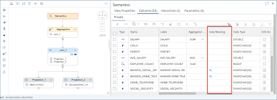
This is the most obvious of the data protection features. This masks out specified parts of data with a pattern using a replacement character. I have applied masking to home telephone numbers and social security numbers.
Figure 1.1: Data Masking on Telephone and Social Security
The masking was applied in the Calculation View in the Semantics, but this can also be done at table level.
Figure 1.2: Data Masking in Calculation Views
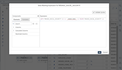
Data Masking is achieved using SQL Expressions
Figure 1.3: Data Masking Expression
2. Differential Privacy
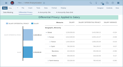
This features adds noise to the specified fields, while still keeping it statistically relevant.
To visualise this, I have used a Geographic Hierarchy, so that you and see how the noise differs within the hierarchy.
Figure 2.1: Differential Privacy: Applied to Salary
The differential privacy parameters that control how much noise and the probability an individual contributes to the result, reside in the anonymization view.
Figure 2.2: Differential Privacy View Definition
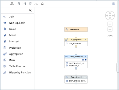
I built a simple calculation view for consumption with SAC, here we use an outer join Geographic Hierarchy
Figure 2.3: Calculation View used to expose Differential Privacy View
3. K-Anonymity
To use the k-anonymity feature we need to define our anonymization rules
◉ Quasi Identifiers
◉ Hierarchies/Groupings
◉ k-anonymity
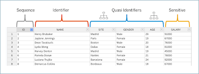
Quasi Identifiers specify which fields could potentially be used to identify individuals. In the dataset below, we chose SITE, GENDER and AGE
Hierarchies/Groupings – How can the quasi identifiers be generalised to allow them to be used. Here we can group ages into age bands, and sites role up a geographic hierarchy. For gender there is no generalisation possible.
K-anonymity, k has been set as 3. This is the minimum number of records needed before we expose the quasi identifiers and sensitive data.
Figure 3.1: Table Data, understand the quasi identifiers
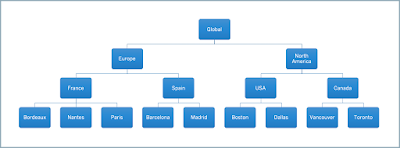
To Generalise the SITE column we used a parent child hierarchy using the structure as below.
Figure 3.2: Site Hierarchy
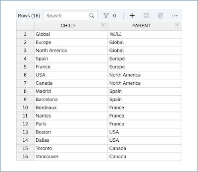
We stored the data for this hierarchy with a parent child structure.
Figure 3:3 Geographic Hierarchy Table
We used the following hierarchy view in the anonymization view.
Figure 3.4: Site Hierarchy View definition
To simplify things, in the first instance I have only specified SITE as the quasi identifier.
I reconstructed the geographic hierarchy to allow the data to be visualised more easily with an SAC story against the anonymization views. In this example I used k=3.
The other parameters are commented out.
Figure 3.5: Anonymization View, k=3, SITE defined as quasi identifier
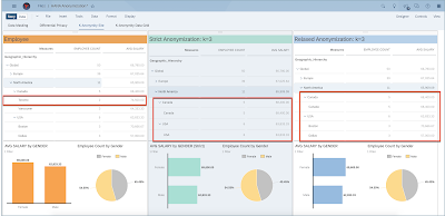
On the left side the Employee column shows the raw data. We can see in Toronto there are only 2 employees which is below our threshold of 3.
In the middle panel, with the strict anonymization applied we can see in the Geographic Hierarchy we no longer see Toronto (as expected), but we also lose Boston and Dallas
On the right side we can have used the more relaxed approach with the “recoding”: “multi_dimensional_strict”
Figure 3.6: k-Anonymity applied to site k=3
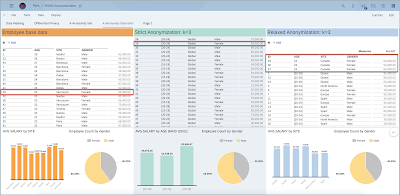
When using multiple quasi identifier in the anonymization view, it makes sense to view the output as a grid. Looking at the dataset we can see ID 29 from Vancouver is anonymized differently depending upon the strict vs relaxed approaches.
Figure 3.7: k-Anonymity with Quasi identifiers Age, Site and Gender




No comments:
Post a Comment