Data science is quite similar to cooking and making your favorite meal. While we can usually simply go to our local supermarket and acquire our raw ingredients, it is often not that easy for a data scientist. Imagen before cooking your favorite meal you didn’t know if the supermarket is open or if the food is even edible. Hence, before the fun part the cooking and eating can start, we need to acquire, organize and structure our data. This is by my experience one of the crucial parts during a Machine Learning use case and usually takes most of the time. Often, the data does not just reside locally in a csv or excel file on our laptop but originally lies in a database like SAP HANA. To work on a database like SAP HANA you usually work with the Structured Query Language (SQL) which is over 40 years old. But as a huge R fan I want to stay in my used environment and not switch back and forth. For example, after the first modeling phase I may have to go back into the data preparation phase to engineer new features. Hence, I want to be more flexible but still use the power of SAP HANA. The R package dbplyr brings both worlds together and is designed to work with database tables as if they were local data frames in R. The goal of the package dbplyr is to automatically generate certain SQL statements for you, focusing on select statements. This means you can continue to use the functions out of the dplyr package with which you are familiar with.
◉ Connect to your SAP HANA through the odbc package
◉ Generate SQL queries directly in RStudio through the dbplyr package
◉ Enable the power of the in-memory database SAP HANA for data preparation
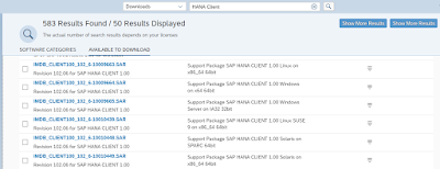
First, we need to connect to our SAP HANA using DBI::dbConnect() through ODBC. To connect to any SAP HANA system, you will need the ODBC client. In case you do not have the HANA ODBC client installed, you can download the client from the SAP Support Launchpad.
What will you learn?
◉ Connect to your SAP HANA through the odbc package
◉ Generate SQL queries directly in RStudio through the dbplyr package
◉ Enable the power of the in-memory database SAP HANA for data preparation
First, we need to connect to our SAP HANA using DBI::dbConnect() through ODBC. To connect to any SAP HANA system, you will need the ODBC client. In case you do not have the HANA ODBC client installed, you can download the client from the SAP Support Launchpad.
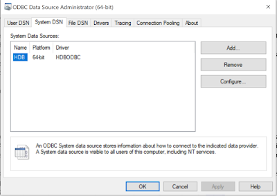
After completing the installation open the ODBC Data Source Desktop app. Then on System DNS choose Add and select HDBODBC.
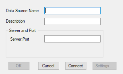
Enter the Data Source Name, Description and Server:Port and press Connect.
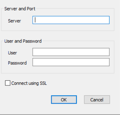
Next, enter your username and password and choose OK.
If you completed the setup successful you will get the following prompt.
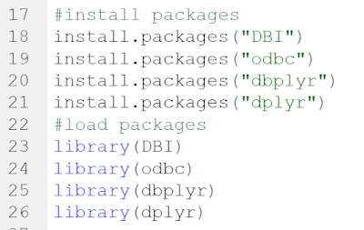
Now, we move into my favorite environment RStudio. The R script is available under the following link. First, we must install the following packages:
Next, we randomly simulate our own data, which of course fits to our cooking theme in this Hands-On tutorial. Therefore, we simulate one data frame(df1) which contains for each customer the bought ice cream sort. In addition, we create one data frame (df2) in which certain customers provided feedback for the ice cream ranging from 1 to 5 with 5 being the highest score. Hence, please execute the following R script:
After simulating our data, we need to connect to our SAP HANA through ODBC and push our data into the database. To create the connection we use the dbConnect() function out of the DBI package. The tutorial under this link really helped to get started. Please make yourself familiar with the odbc() and dbConnect() functions. Then provide your credentials into the provided R script and execute the following lines:
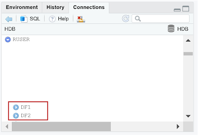
After refreshing you should see the two datasets DF1 and DF2 under the connections, which are now residing in our SAP HANA. We are able to control this directly in RStudio.
Further, we use the tbl() function to create a reference to these tables. Then we print the results to our console, which looks like a regular tibble.
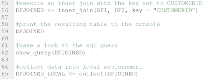
In the next step we create an inner join to combine the two datasets through the customer ID. After joining the two tables we can look at the SQL query or load the data in our local RStudio environment. We can therefore execute all the computational costly data preparation steps directly in SAP HANA using the power of our in-memory database and then only collect our final dataset.
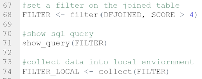
The dplyr package provides many functions to prepare and transform our data. Of course, this is just the tip of the iceberg in this Hands-On tutorial. Hence, as a second example we will filter our joined dataset focusing on all the customers which gave our ice cream a score higher than 4. Therefore, please execute the following R script:
As we can see in the table our ice cream Chocolate Fudge Brownie was scored the highest from two customers.
Furthermore, you may of course copy the SQL query acquired through the show_query() function and execute it directly in SAP HANA Studio.






No comments:
Post a Comment